Ultrasonic 3D Tracking
Introduction
In the Ultrasonic Ranging project, we showed how to obtain range, i.e., distance estimates from ultrasound measurements. In many applications, though, it is desirable to track the 3D coordinates of the measured target, either cartesian or spherical, which poses several challenges. Other sensing technologies, such as Radars and GPS, use antenna arrays, beamforming, trilateration and time-synchronization for this purpose. However, because of the limitations due to the ultrasound wavelength and the mounting of speakers and microphones, many algorithms cannot be applied to the measurements obtained with the SensEdu platform, as they lead to large tracking errors. In order to overcome these issues, an extended version of the SensEdu PCB has been developed, featuring 8 microphones placed further apart with respect to the standard PCB version. In this project, we show the implementation of a live 3D tracking framework using this board, different signal processing techniques and an Extended Kalman Filter (EKF)
The Extended SensEdu
The primary factor influencing the tracking error is the distance between the microphones and the speaker. Additionally, increasing the number of microphones improves performance. The updated system features a larger physical layout, measuring 20x20 cm, compared to the original compact design of 5x5 cm. This revised configuration includes eight microphones strategically positioned: four located at the corners (with a 13 cm distance from the speaker) and four placed at the center of each side (with a 9 cm distance from the speaker). The following picture shows the front and back layouts of the board:
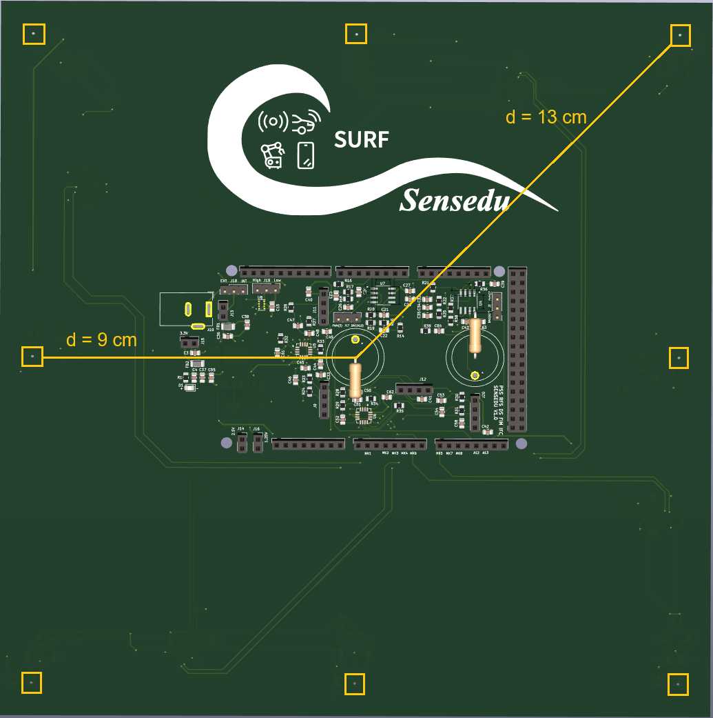
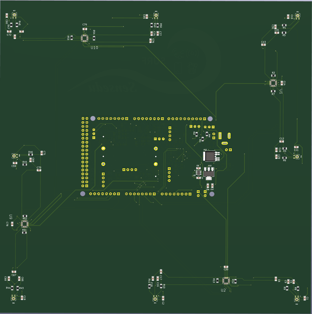
To further enhance performance, two additional amplifiers have been integrated, each connecting two microphones in a single two-channel configuration. The schematics are available in the PCB section of the documentation.
This PCB has been designed extending a previous version of the main SensEdu board, therefore you might notice some differences in the layout. For the purposes of the 3D tracking project, these differences are irrelevant.
Signal Processing and EKF
The data acquisition process shares the initial parts with the Ultrasonic Ranging project, namely the transmission of a sine-burst wave through the DAC, the reception, rescaling and filtering of the 16-bit audio signals from the ADCs, the cross-correlation and the robust peak search algorithm to obtain the distance of the target with each microphone. We will use these distances later in the measurement update step of the EKF. The filter is needed to process the computation of cartesian coordinates from distance estimates. The cartesian coordinates represent the position of the object in the 3D space and, together with its velocity, form the target’s state. When talking about target tracking, we want to estimate its state live at each time step, so that we can predict where it will move next, and correct our prediction based on the new measurements we receive.
State Propagation (Prediction)
We model the target dynamics in a generic fashion, independent of specific devices. Generally, random noise affects the position of a target object, acting as an external driving acceleration force that changes velocity and position of the object, which are the state variables that need to be tracked. The velocity of the object is represented by a 3D Brownian motion \(\boldsymbol{W}_v(t)\), and the position of the object is represented as an integral over the Brownian motion (also known as a Wiener process). It is assumed that each sample of \(\boldsymbol{W}_v\) is statistically independent and distributed as \(\mathcal{N}(0, t-s)\) where \(t\) is time and \(s\) is a specific time for one sample, with \(0\le s < t\). At each time, the 3D velocity \(\boldsymbol{V}(\tau) = [V_x(\tau),V_y(\tau),V_z(\tau)]^T\), and the 3D position \(\boldsymbol{X}(\tau) = [x(\tau), y(\tau), z(\tau)]^T\) terms can be computed solving the stochastic differential equations:
\[\begin{align} \boldsymbol{V}(\tau) &= \boldsymbol{V}_0 + \boldsymbol{\sigma}_v \boldsymbol{W}_v(\tau) \\ \boldsymbol{X}(\tau) &= \boldsymbol{X}_0 + \int_0^\tau\boldsymbol{V}(s)ds \end{align}\]where \(\tau \in \mathbb{R}^+\), and \(\boldsymbol{V}_0 = \boldsymbol{V}(0)\) and \(\boldsymbol{X}_0 = \boldsymbol{X}(0)\) are constant and represent the initial velocity and position of the object, respectively. The target is observed in discrete time: at each time step \(t\Delta\tau\), the system states can be represented with the following recursive relations:
\[\begin{align} \hat{\boldsymbol{V}}_t &= \hat{\boldsymbol{V}}_{t-1} + \boldsymbol{\alpha}_t \\ \text{where } \boldsymbol{\alpha}_t &= \boldsymbol{\sigma}_v(\boldsymbol{W}_v(t\Delta\tau)-\boldsymbol{W}_v((t-1)\Delta\tau))\\ \\ \hat{\boldsymbol{X}}_t &= \hat{\boldsymbol{X}}_{t-1} + \hat{\boldsymbol{V}}_{t-1}\Delta\tau + \boldsymbol{\beta}_t \\ \text{where }\boldsymbol{\beta}_t &= \boldsymbol{\sigma}_v\int_{(t-1)\Delta\tau}^{t\Delta\tau}(\boldsymbol{W}_v(s)-\boldsymbol{W}_v((t-1)\Delta\tau))ds \end{align}\]The increments of the Brownian motion are represented as \(\boldsymbol{U}_t = [\boldsymbol{\alpha}_t, \boldsymbol{\beta}_t]^T\). Each instance is modeled as a multivariate normal distribution that has zero mean and covariance matrix (computed with Ito’s Lemma):
\[\begin{equation} \boldsymbol{Q} = \Delta\tau \begin{bmatrix} \boldsymbol{\sigma}_v^2\boldsymbol{I} & \frac{\boldsymbol{\sigma}_v^2}{2}\Delta\tau\boldsymbol{I} \\ \frac{\boldsymbol{\sigma}_v^2}{2}\Delta\tau\boldsymbol{I} & \frac{\boldsymbol{\sigma}_v^2}{3}\Delta\tau^2\boldsymbol{I}\\ \end{bmatrix} \end{equation}\]with \(\boldsymbol{I}\) being a three-dimensional identity matrix. The final system state propagation is given by:
\[\begin{align} \hat{\boldsymbol{S}}_t = \boldsymbol{F}\hat{\boldsymbol{S}}_{t-1} + \boldsymbol{U}_t \end{align}\]where \(\hat{\boldsymbol{S}}_t = [\hat{\boldsymbol{V}}_t, \hat{\boldsymbol{X}}_t]^T\) is the system state vector linearly propagating with:
\[\begin{equation} \boldsymbol{F} = \begin{bmatrix} \boldsymbol{I} & 0 \\ \Delta\tau\boldsymbol{I} & \boldsymbol{I} \end{bmatrix} \end{equation}\]Measurement Update (Correction)
When the measurements arrive, we can use them to “correct” the previous estimation. Since we get 8 distance measurements (one from each microphone), we need to find a way to compute \(\boldsymbol{X}\) from the distance \(\boldsymbol{D}\). Let \(\boldsymbol{r}\) represent the distance vector between the object \(O\) and the speaker \(S\) with coordinates \((x_s, y_s, z_s) = (0, 0, 0)\), serving as the origin of the local coordinate system. Let \(\boldsymbol{m_i}\) represent the distance vector between the speaker and the \(i\)-th microphone, with \(i \in \{1, 2, \dots, 8\}\), and \(\boldsymbol{r_i}\) the distance vector between the object and the \(i\)-th microphone. Then:
\[\begin{equation} \boldsymbol{r} + \boldsymbol{r_i} = \boldsymbol{m_i}, \quad i \in \{1, \dots, 8\} \end{equation}\]The distance value \(\boldsymbol{D_i}\) for each microphone is computed from the time-of-flight (TOF) and is the sum of the norms of \(\boldsymbol{r}\) and \(\boldsymbol{r_i}\). Therefore:
\[\begin{equation} \|\boldsymbol{r}\| + \|\boldsymbol{r_i}\| = \|\boldsymbol{r}\| + \|\boldsymbol{m_i} - \boldsymbol{r}\| = D_i = ToF_i \times c, \quad i \in \{1, \dots, 8\} \end{equation}\]where \(c = 331 \, \mathrm{m/s} \times \sqrt{1 + \frac{T(^\circ C)}{273.15}}\) is the speed of sound in air (roughly 343 \(\mathrm{m/s}\) in normal operating conditions at 20\(^\circ C\)).
The main challenges lie in the fact that both \(\boldsymbol{r}\) and \(\boldsymbol{r_i}\) are unknown, and that the physical placement of the sensors exceeds the signal wavelength. The EKF leverages the temporal consistency of the measurements, so the equation above represents the measurement function \(h(\hat{\boldsymbol{X}}_t)\) for the residual calculation in the update step of the filter:
where \(\boldsymbol{\hat{S}}\) is the six-elements state vector with position and velocity in 3D, \(\nu\) is the measurement noise and \(\boldsymbol{K}\) is the Kalman gain matrix.
Showcase
This section shows two example results obtained with the 3D tracking algorithm for a “squared” and a “spiral” trajectory. Actual performances depend on the selected number of samples, sampling frequency, number of peaks per microphone (MAX_PEAKS), as well as on the particular shape/material of the target and its motion.
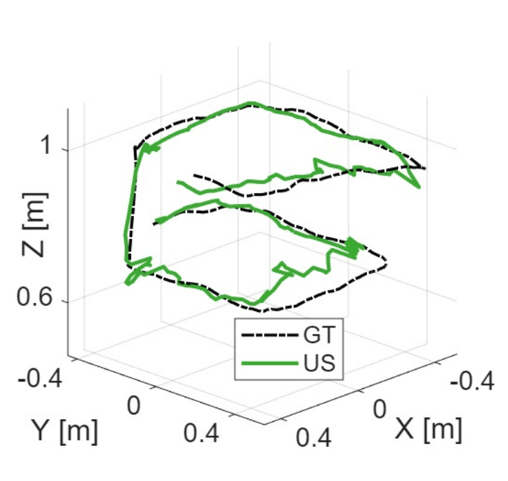
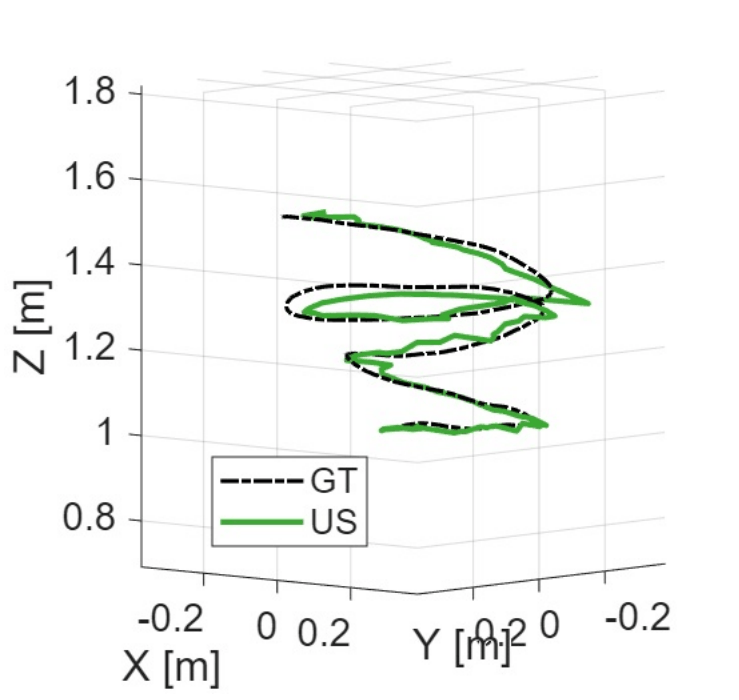
The Ground Truth (GT in the plots) has been obtained with the Motion Capture system Optitrack. Notice that the position computation with the ultrasound sensors (US in the plots) is affected by errors which degrade the accuracy, but the object is consistently tracked at all times. Some error is also due to the poorly measurable offset between the Optitrack marker (the point actually measured in GT) and the reflection point of the target for the US sensors. The obtained tracking data match the real trajectories with errors in the order of a few centimeters, which can be considered very acceptable given the overall low-cost and simplicity of the sensing hardware.